Structural data can be imported from
both clipboard and files or from previously saved Open Plot files.
When importing data copied from a
spreadsheets or loaded from a text file, the first step is to properly organise the
dataset.
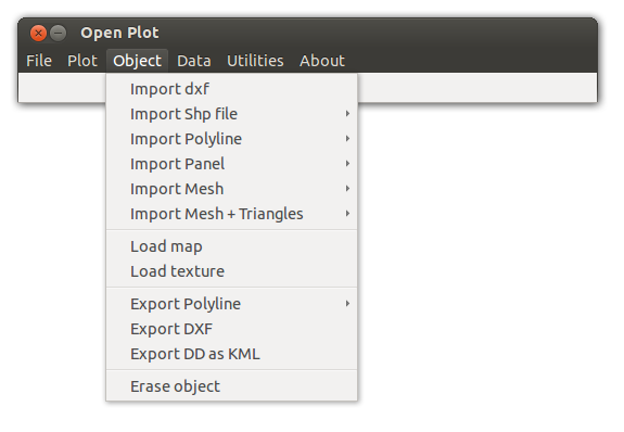
Many
Basic 3D objects and all the
complex objects are imported both from clipboard and from
external files, via the Object
sub-menu
Importing structural data
How to organise
structural data
Data must be organised as follow:
Rows = elements.
Columns = element's attributes.
Eventually,
the first row can contain the columns header.
Numeric
fields rigorously do not have to include non numeric characters.
As
an example, the azimuth must be expressed as a number ranging between
0 and 360. Expressions like N180º or N56E will return an azimuth =
0.
For
a given element, when the value of an attribute is not defined the
corresponding field must be empty.
Example
spreadsheet with correct data organization
| Data Type |
Azimuth |
Dip |
Pitch |
Spacing |
| Fault |
123 |
57 |
24 |
477 |
| Joint |
345 |
83 |
|
35 |
| Fault |
133 |
48 |
12 |
|
Example
of spreadsheet with incorrect data organization
| Data Type |
Azimuth |
Dip |
Pitch |
Spacing |
| Fault |
123 |
57 |
24 |
477 mm |
| Joint |
345 |
83 |
-
|
35 |
| Fault |
133 |
48 |
12 |
/
|
In
the correct table joint has not an associated pitch value.
Analogously, the second fault has not an associated spacing value.
In
the Incorrect table, the character “–“
in the pitch field of the joint will return a pitch = 0. Spacing of
both faults will be set = 0, as non numeric characters are present.
If
data are loaded from a text file, each row must contain the same
number of fields.
Correct
data organization with fields divided by commas.
Data
type, azimuth, dip, Pitch, spacing
Fault,123,57,24,477
Joint,345,83,,35
Fault,133,48,12,
Data
in the Joint row will be read as follow: Data type=Joint;
Azimuth=345; Dip = 83; Pitch = EMPTY (two commas with no character in
between); spacing = 35. Analogously, for the second fault, data will
be read as follows: Data type=Fault; Azimuth=133; Dip =48; Pitch =
12, Spacing = EMPTY.
Incorrect
data organization
Data
type, azimuth, dip, Pitch, spacing
Fault,123,57,24,477
Joint,345,83,35
Fault,133,48,12
Data
in the Joint row will be read as follow: Data type=Joint;
Azimuth=345; Dip = 83; Pitch = 35. The character after 35 is an
“enter”. This implies that the joint row is characterised by 4
fields, while the first fault is characterised by 5 fields. Due to
this the software will stop reading the file (eventually it will
crash). Analogously, for the second fault data will be loaded as
follows: Data type=Fault; Azimuth=133; Dip =48; Pitch = 12; the
character after 12 is an “enter” and the software will stop
reading.
Faults
sense of slip
During
data import, fault slickenline can be imported as both pitch or
slickenline
azimuth. Regardless of this, if at least one of these two field is
not empty, the software will compute the values of: slickenlines
pitch and azimuth and of rotax (slip normal) azimuth and dip. If not
present in the imported dataset, these fields are automatically
added.
In
the field defining the fault's sense of slip, English nomenclature
must be adopted.
A
fault is considered:
-
Normal when the first two letters are NO
or NR
-
Reverse, when the first two letters are RE
or
RV
-
Left-lateral, when the first two letters are LE
or
LL
-
Right-lateral, when the first two letters are RI
or
RL
This
check is not case sensitive.
In
all the other cases the sense of slip is considered undetermined
Import from Clipboard
(see the movie)
This
allows to import data copied from a spreadsheet. Open
the spreadsheet and copy
the selection containing data.
From the main
window of Open Plot select:
File
→
Import from Clipboard
If
data are correctly loaded it will be asked if data include
an header (if it is the case it is assumed that the column header
locates in the first row).
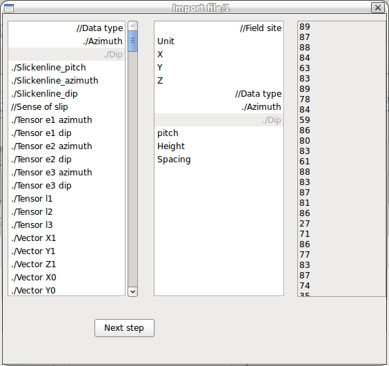
A
new window will open up.
In
the first and second list-boxes on the left are listed the “software
defined” and the “user defined”
fields, respectively. In the third list-box are listed the values
associated with the selected “user defined” field.
When
possible, select the “user defined” field and double click the
corresponding
“software defined” field. This substitutes in the header the
“user defined” field name with the “software defined” field
name.
When
all
the possible substitutions have been done click “Next step”.
 The
window will enlarge and it will be asked to specify for each
unassigned field if it is a Value field (numeric field, like spacing,
aperture) or a Class field (alphanumeric field, like author, year...)
Double-click
on the unassigned fields to “assign” them and then click “Next
step”.
The
window will enlarge and it will be asked to specify for each
unassigned field if it is a Value field (numeric field, like spacing,
aperture) or a Class field (alphanumeric field, like author, year...)
Double-click
on the unassigned fields to “assign” them and then click “Next
step”.
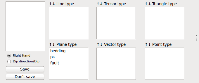
 In
the new window it will be asked to specify, for each element in the
“Data type”
field, if it is a Line, a Plane, a Tensor, a Vector or a Triangle.
Select/multiselect
the element/s and, holding the keyboard space bar pressed, drag
the element/s in the corresponding type list-box. If
planar elements are present, it must be specified if the azimuth
field corresponds
to the plane dip direction or to the plane strike.
In
the new window it will be asked to specify, for each element in the
“Data type”
field, if it is a Line, a Plane, a Tensor, a Vector or a Triangle.
Select/multiselect
the element/s and, holding the keyboard space bar pressed, drag
the element/s in the corresponding type list-box. If
planar elements are present, it must be specified if the azimuth
field corresponds
to the plane dip direction or to the plane strike.
 In
this
window, a given type list-box is enabled only if loaded elements
include fields that are required by that type:
To
define
a Line and a Plane the azimuth and dip fields must exist.
To
define a Tensor the azimuth and dip fields of the three eigenvectors
must exist (the eigenvalues are optional).
To
define a Vector the three coordinates of the starting and ending
points must exist.
To
define a Triangle the three coordinates of the three points must
exist.
Notice
that for Vectors and Triangles the software will automatically
compute the azimuth and dip values.
Finally
you
can decide to save the data as *.stv file or continue without saving.
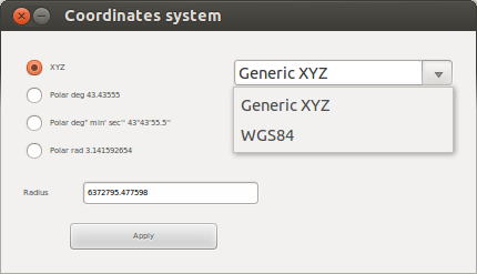
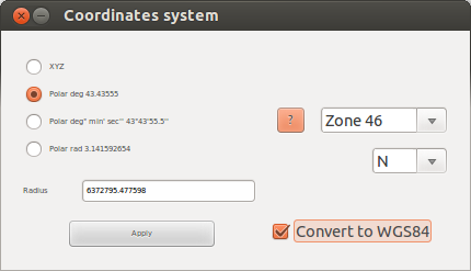
If
X,Y, and Z coordinates have been provided, it will be asked to specify
if these coordinates are in Geographyc or Cartesian
system.
Allowed cartesian systems are Generic XYZ and WGS84, in the second case
it is assumd that the provided values are in meters.
Polar
coordinates will be tranfsormed into WGS84 (Zone is required).
In
this
window, a given type list-box is enabled only if loaded elements
include fields that are required by that type:
To
define
a Line and a Plane the azimuth and dip fields must exist.
To
define a Tensor the azimuth and dip fields of the three eigenvectors
must exist (the eigenvalues are optional).
To
define a Vector the three coordinates of the starting and ending
points must exist.
To
define a Triangle the three coordinates of the three points must
exist.
Notice
that for Vectors and Triangles the software will automatically
compute the azimuth and dip values.
Finally
you
can decide to save the data as *.stv file or continue without saving.
If
X,Y, and Z coordinates have been provided, it will be asked to specify
if these coordinates are in Geographyc or Cartesian
system.
Allowed cartesian systems are Generic XYZ and WGS84, in the second case
it is assumd that the provided values are in meters.
Polar
coordinates will be tranfsormed into WGS84 (Zone is required).
 Import from File (see the movie)
The
procedure
is the same as described in the Import
from
clipboard, with the exception of the following initial steps.
From
the main window of Open Plot select: File → Import from File and
select the file.
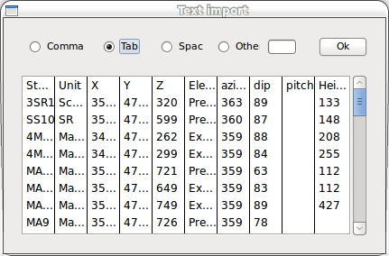
Import
from File needs the separator definition, which must be specified
in this window that will automatically open.
 Importing basic 3D
objects
and complex objects
Importing basic 3D
objects
and complex objects
 Import
dxf presently reads only the following DXF types: "POLYLINE" and "3Dface".
Import shape files
(*.Shp), allows reading X and Y coordinates and transforms elements
into either 2D vectors or 2D polylines (tested on Quantum Gis shape
files).
Import
dxf presently reads only the following DXF types: "POLYLINE" and "3Dface".
Import shape files
(*.Shp), allows reading X and Y coordinates and transforms elements
into either 2D vectors or 2D polylines (tested on Quantum Gis shape
files).
Import polyline and Import panel
allow to read a sequence of X,Y,Z values, both from a text file and
copied from the
clipboard, and transform them into a polyline and
panel, respectively.
Import Mesh allows to load XYZ
surfaces and convert them into triangular meshes.

import Mesh > *.xyz: read files including an organised
sequence of X,Y, and Z coordinates (and eventually R,G,B values), like
the following:
335574.000,4799414.000,316.129,255,255,255
335574.000,4798578.214,298.810,255,255,255
335574.000,4797742.429,291.856,255,255,255
335574.000,4796906.643,311.637,255,255,255
335574.000,4796070.858,334.093,255,255,255
335574.000,4795235.072,334.635,255,255,255
335574.000,4794399.286,335.162,255,255,255
335574.000,4793563.501,369.754,255,255,255
335574.000,4792727.715,413.278,255,255,255
335574.000,4791891.930,427.381,255,255,255
Tested on Global Mapper files
import Mesh > GoCad
*.ts: import surfaces
in GoCad TS format.
import Mesh > Earth
Vision: import surfaces
in Earth Vision format.
import Mesh >
Quantum Gis Interpolation File: import a QGis interrpolation file.
import Mesh >
*.obj: import triangular meshes in wavefront
format.
Tested on OBJ files made with Agisoft PhotoScan. If the file includes also a
texture map, it is uploaded and associate to the mesh.
For
all the import mesh, an "+ triangles" option exists. This option allows
to import the triangles of a mesh as independent objects separated from
the native mesh. For these triangles, azimuth and dip are automatically
computed and many plot/selection operations are available for them
Load
Map: load an image and georeference it (asking
the coordinate system), to later drape it onto a mesh.
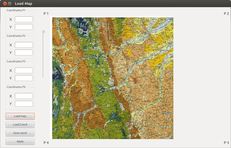 Manually inserting the coordinates of 3 of the 4 vertex is required for
georeferentiation. Alternatively, if the image has an associated *.jgw
file, coordinates are automatically read from it.
From version 2013-GL-00, which uses OpenGL
libraries, images that are not properly dimensioned, must be resampled
and their dimensions (in pixels) are set to the nearest power of two
value (i.e. 256, 1024, 2048, 8192). Accordingly, in order to not reduce
the image quality, it is highly recommended to upload images having
native power-of-two dimensions.
Manually inserting the coordinates of 3 of the 4 vertex is required for
georeferentiation. Alternatively, if the image has an associated *.jgw
file, coordinates are automatically read from it.
From version 2013-GL-00, which uses OpenGL
libraries, images that are not properly dimensioned, must be resampled
and their dimensions (in pixels) are set to the nearest power of two
value (i.e. 256, 1024, 2048, 8192). Accordingly, in order to not reduce
the image quality, it is highly recommended to upload images having
native power-of-two dimensions.